Technical information
This section of the documentation contains information that may be required by advanced users who wish to obtain a thorough understanding of the operation of the software.
The grain measurement procedure
The image processing and analysis procedures utilised by Digital Gravelometer to identify and measure the grains in images are described in detail by Graham et al. (2005a; b). The procedures have been subject to intensive testing to define those internal parameters that provide optimal results. Whilst it is not essential to fully understand these procedures in order to be able to use the software, it is recommended that a thorough understanding is achieved before modifying the values of these parameters.
Stages in the grain identification and measurement procedure
The identification and measurement of grains by Digital Gravelometer is an eight-stage process. The individual steps, and the significance of the parameters they use, are described here. Changes to the values of the parameters specified may by made in the Processing options dialogue box.
Stage 1: Convert to grayscale
The colour image is first converted into a grayscale (intensity) image. There is an option to view the grayscale image in the Output options dialogue.
Stage 2: Apply correction for radial lens distortion
If the user has specified that radial lens distortion should be corrected, the grayscale image is modified to incorporate this correction.
Stage 3: Apply a projective transform
A projective transform is applied to the image to correct for the axis of the camera not being help perfectly vertically above the centre of the sample patch. This transform resamples the image and requires the specification of a sampling resolution (the number of pixels per mm). An appropriate value is calculated automatically by the software to keep the image resolution approximately constant. However, it is possible for the user to specify a different value. This is not recommended as it will result in either a loss of image resolution or the sampling of the image at a higher resolution than that of the original image (resulting in longer processing times without any improvement in the quality of the results). The output of this stage is a rectified grayscale image. There is an option to view the rectified image in the Output options dialogue.
Stage 4: Identify the grains in the image
This stage converts the grayscale image into a binary (black and white) image in which the grains are represented by white and the interstices by black. This stage is itself composed of several steps:
- Noise in the image is reduced by the application of a median filter. The default filter size is 5 x 5 pixels, but this may be altered by the user. A larger filter reduces the noise in the image but results in some blurring.
- The interstices are enhanced by the application of a morphological bottom-hat filter. The default filter ('structuring element') is a disk with radius 15 pixels, but the size may be altered by the user. The objective of the filter is to enhance small dark areas in the image that represent interstices without enhancing large dark areas that may be dark coloured grains. Increasing the size of the structuring element may increase the number of grains excluded, whilst decreasing its size may result in inadequate enhancement of some interstices.
- The enhanced image is converted into two binary images by thresholding at two different intensity values. The values are defined as percentiles of the intensity-frequency distribution and may be modified by the user. Threshold 1 is designed to identify all of the interstices in the image, but is also likely to include some intra-grain noise. Threshold 2 is designed to identify only the very darkest points in the image that definitely represent interstices. The two binary images are combined so that a third binary image is created that includes only those interstices in the first image that are connected to those in the second.
There is an option to view the result of the initial segmentation in the Output options dialogue.
Stage 5: Separate touching grains
It is common for those regions that represent grains in the resulting binary image to be connected. The binary image is further segmented by the application of a watershed transform. This may result in significant oversegmentation of the image. An intermediate step in the watershed transform is smoothed by the application of an h-minima transform. The intensity of this smoothing is controlled by the minima suppression parameter, the default value of which is 1. Reducing this value will result in increased oversegmentation of grains, whilst increasing it may result in the failure to separate touching grains. The output from the watershed segmentation is a final binary representation of the grains in the original image. There is an option to view the result of the watershed segmentation in the Output options dialogue.
Stage 6: Select the grains to measure
Those grains that lie within the sampling area defined by the control points are now selected for measurement. Because either including or excluding all of the grains intersecting the boundary of the sampling area will result in a size bias (against and in favour or large grains respectively), it is best to include grains intersecting half of the perimeter and exclude the rest. By default, those grains lying along the top and left edges of the sampling area are included. This may be changed by the user. The output of this step is a binary image containing only those images to be measured. There is an option to view the result of the application of the boundary rules in the Output options dialogue.
Stage 7: Measure the grains
The selected grains are now measured. Information is recorded about grain size, orientation, shape and area. At this stage, the grain sizes are specified in pixels.
Stage 8: Convert grain sizes to millimetres
The final stage is to convert the measured grain sizes into millimetres using the known scale of the imagery.
Square-hole sieve correction
Definition of the b-axis
The most usual index of grain size employed by sedimentologists is the length of the b-axis. This is usually defined as the longest dimension perpendicular to the long (or a-) axis. In an image, the conceptually equivalent index is the longest dimension perpendicular to the apparent long (major) axis of the grain (the minor axis). This may not be exactly the same as the true b-axis because the a-b plane may not be perfectly parallel to the plane of the image. In practice, this definition is difficult to apply and it is usual within the image-processing community to define the minor-axis length as the minor axis of the ellipse that has the same normalized second central moments as the region. Graham et al. (2005a) demonstrated that the use of this definition makes no significant difference to the grain-size distribution obtained.
Sediment grading with sieves
The most usual method of measuring the b-axis of sediment grains is to grade them into classes using sieves, which commonly have square holes. However, the sieve on which a grain is retained is a function not only of its b-axis, but also its c-axis (the axis that is perpendicular to both the a- and b-axes). This is because a grain with a large b-axis and small c-axis may present itself to the sieve hole diagonally and pass through a hole that is nominally smaller than the true b-axis of the grain. For platy grains, the net result is an apparent coarsening of the grain-size distribution compared to that which would be obtained by individually grading each grain by measuring its b-axis with a ruler.
Square hole sieve correction
Because the b-axis measurement made by the Digital Gravelometer is more analogous to that made with a ruler than with a square-hole sieve, it is necessary to adjust the measurements made by the software if they are to be directly compared to sieve-derived data. Such an adjustment has been presented by Church et al. (1987):
![]()
where the ratio of square-hole sieve size and true b-axis (Ds / b) is related to flatness (c / b). This relation requires knowledge of the flatness of each grain in order to calculate a correction factor for each. Whilst it is not possible to directly determine the flatness of grains from an image, it is relatively quick to characterise the typical grain flatness for a particular sediment body by measuring a sample of, perhaps, 100 grains in the field. This may then be used to calculate a correction factor which may be used to adjust the sizes of all of the grains measured by the software. In practice, it has been determined that the grain-size distribution is insensitive to the precise value of the correction applied and a correction factor of 0.79 (corresponding to a mean flatness of 0.51) has been shown to give good results even for sediments with an obvious difference in grain shape.
Correction of radial lens distortion
Radial distortion is the most significant of the lens distortions associated with non-metric cameras. The distortion varies between cameras and at different focal lengths. Whilst the effect of radial distortion on the derived grain-size distribution is likely to be small, it may be significant for some cameras at certain focal lengths.
Digital Gravelometer provides the capability to both apply a correction for radial distortion during the grain measurement process and to determine the appropriate correction coefficients required for particular cameras and focal lengths.
Deriving radial lens correction parameters
If a radial correction is to be applied during the grain measurement procedure, a lens-correction parameters file must be created for the camera used to collect the sample images. Creation of the parameters file is a two stage process:
- images must be taken in the laboratory from which the parameters may be determined
- the parameters must be derived for the images using the software.
Laboratory image collection
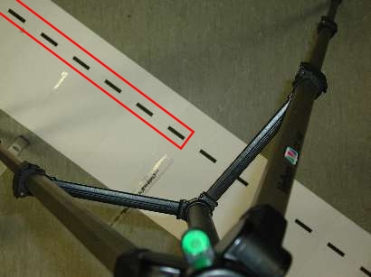
The first stage is to collect a series of images with a single digital camera at a variety of focal lengths. Each image must contain equally spaced markers running in a straight line between the top-left and bottom-right corners. The procedure is:
- On a flat surface, set up the camera on a tripod with the camera pointing vertically down. It is essential that the axis of the camera is vertical (use of a spirit level is recommended). The camera height should be approximately the same as that used to collect sample images in the field.
- Lay a long object, on which there are equally spaced marks, diagonally across the field of view (from top-left to bottom-right). The object may be a tape, a surveying staff or paper with printed marks. It is essential that the alignment of the markers runs perfectly from corner to corner. In addition, one of the markers must be located precisely in the centre of the camera's field of view (directly on the axis of the camera). It must be possible to see all of the markers between the centre and top-left corner of the image.
- Photograph the object at a range of focal lengths.
- Transfer the images to the computer on which Digital Gravelometer is installed.
An example of the type of image required is given below. All of the markers in the area outlined in red must be visible in the image. In this example, the markers are 5 cm black bars printed on a strip of paper.
 Derivation of radial distortion parameters within Digital Gravelometer
Because it is known that the markers in each image are equidistant, it is possible to use them to determine the nature of any radial distortion within each image. This is undertaken using the Define lens-correction parameters dialogue accessed from the menu. Instructions may be found in the Reference (lens correction) section of this documentation.
Successful addition of multiple images requires that the software is able to determine the focal length at which each image was taken. All modern digital cameras store this information in the header information of each image, but it may be destroyed if the image is modified in any other software prior to being imported into Digital Gravelometer. If header information is not found, it is only possible to calculate one set of correction parameters in each parameters file. In this case, it is recommended that the focal length used should be approximately the same as that used to collect sample images in the field (i.e. approximately the same area should be photographed from the same height).
Applying a radial lens correction during grain measurement
The radial lens correction is applied to images during the grain measurement procedure. The appropriate radial lens correction parameters file may be selected from the Processing options dialogue accessed by clicking the appropriate button from the Measure grains dialogue. Further information may be found in the Reference (measure grains) section of this documentation.
If a radial correction is to be applied, it is essential that the parameters file used was created for the particular camera employed to collect the sample images.
Calculation of grain-size distributions and statistics
Grain-size distributions and statistics may be calculated and presented in a variety of different ways. When comparing grain-size information it is essential to ensure that like is compared with like. This section presents a variety of technical information to help the user make informed choices about the presentation of their grain-size information.
The settings described below may be modified in the Report options dialogue (accessed from the menu).
Size distribution calculations
Percent finer vs percent coarser
Grain-size distributions are commonly presented as cumulative curves showing the proportion of grains finer or coarser than a given size. Digital Gravelometer provides the option of presenting the distribution in either way. Whilst the difference is essentially cosmetic, the user should be aware that low value percentiles represent the smallest grains for percent-finer-than distributions and the largest grains for percent-coarser-than distributions. Note that this option does not affect the derived graphical statistics that, for consistency with the original literature (Folk and Ward, 1957), are always calculated on a percent coarser-than basis.
Grid-by-number vs area-by-number distributions
Digital Gravelometer allows grain-size distributions to be presented to be compatible with data collected on an area-by-number basis (e.g. a paint-and-pick sample) or a grid-by-number basis (e.g. a Wolman sample). Selection of the appropriate option is critical because the shape of the distribution is significantly different for the two methods. Users who are are unsure which option is appropriate for a particular application are advised to contact an experienced practitioner.
Digital Gravelometer calculates distributions on an area-by-number basis simply based on the b-axis measurements of every grain. Using this method, every grain in the distribution carries the same weighting in the grain-size distribution. It is equivalent to a paint-and-pick sample where every grain in a fixed area is sampled and the probability of sampling any particular grain is the same (i.e. 1).
Grid-by-number distributions are conventionally generated by sampling grains on a regular grid laid across the surface to be sampled (e.g. a Wolman grid sample). In this type of sample, the probability of sampling a particular grain is proportional to its area. Digital Gravelometer generates distributions equivalent to those produced by grid sampling in a similar way to the method of Sime and Ferguson (2001). Each grain is weighted based on its area before calculating the distribution parameters. Although it produces results that are equivalent to a grid-based sample, the method uses every grain in the sampling area and it is therefore possible to derive a sample from a much smaller area than would be possible using a conventional grid-based sampling method (in which only a small proportion of the grains in the sampling area is actually sampled).
Calculation of percentiles
The user has the option of including information about various grain-size percentiles (the grain size below or above which a certain percentage of the distribution lies) in the report. The conventional method of calculating percentiles (used when grain-size information is only available for size classes, such as for sieve-derived data), is to obtain the percentiles at each size-class boundary and apply a linear interpolation to obtain intermediate percentiles. Because Digital Gravelometer measures the size of every grain individually, it is able to calculate exact percentiles without the need for interpolation. This is equivalent to having an infinite number of size classes in the conventional approach. In practice, the difference between the two methods is likely to be small except at the extremes of the size distribution.
Calculation of distribution statistics
Distribution statistics
Digital Gravelometer is able to calculate grain-size distribution statistics using both graphical and moments methods.
Graphical statistics are based on percentiles of the grain-size distribution. Such percentiles were traditionally determined manually from a hand-drawn cumulative grain-size distribution curve produced from the number of grains in individual sieve-size classes. Graphical statistics have the advantage that they are not sensitive to the tails of the distribution (which are commonly relatively poorly constrained). The statistics calculated by Digital Gravelometer are the inclusive graphical statistics of Folk and Ward (1957). Because Digital Gravelometer is able to determine the size of every grain individually (rather than just the class in which it lies) it is able to determine the percentiles of the grain-size distribution very precisely without interpolation. Because the percentile values on which they are based are calculated very precisely, the graphical statistics presented by Digital Gravelometer may differ slightly from those presented by other software packages.
Moment statistics are based on the entire grain-size distribution and are particularly simple to calculate using a computer without the need to obtain grain-size percentiles. Their advantage over graphical statistics is that they utilise the entire grain-size distribution. The corollary is that they are inappropriate where the tails of the distribution are inadequately specified. Moment statistics are conventionally calculated from sieve-derived data based on the proportion of grains in each sieve class. Using this approach, the number of classes used affects the values obtained. Folk (1966) demonstrated that the sorting is over predicted when a small number of classes are used. Because Digital Gravelometer measures the size of every grain individually, it is possible to calculate the moment statistics directly from the grain sizes. This is equivalent to using an infinite number of sieve classes. The moment statistics produced from classified grain sizes should be considered an approximation of the true statistics as provided by Digital Gravelometer.
The user may choose to specify that both the moment and Folk and Ward statistics be calculated logarithmically (based on a log-normal distribution with either Phi or Psi units) or geometrically (based on a log-normal distribution with mm units). Additionally, the moment statistics may be calculated arithmetically (based on a normal distribution with mm units). This final option is rarely used, but is provided for comparison with the output of some Coulter sizing instruments (Blott and Pye, 2001).
There is some confusion in the literature over whether grain-size statistics should be calculated on the basis of cumulative percent finer or coarser distributions. Unfortunately, the two approaches give different results for some of the statistics, resulting in different inconsistent use of the terms 'positive' and 'negative skewness'. For consistency with the original literature (e.g. Folk and Ward, 1957), the statistics presented by Digital Gravelometer are always calculated on a percent coarser-than basis. A note indicating that positive skewness represents fine skew (i.e. a tail of fine particles) is included in the reports generated by the software.
Export file format
The menu provides the facility to export information about each measured grain for analysis in other software packages. Data are exported in a comma-separated variable (*.csv) file. CSV is a widely supported standard for data files and can be imported by many spreadsheet and statistical packages or by a text editor or word processor (see the File types section of the documentation for further information).
The precise format of the exported file depends on whether the user chooses to export data for images individually or to aggregate them.
Individual
If the user chooses to export the data for each image individually the file is formatted as follows:
| Image filename:, | filename_1 | <newline> | |
| Site name:, | sitename_1 | <newline> | |
| Site ID:, | siteID_1 | <newline> | |
| Image filename:, | filename_2 | <newline> | |
| Site name:, | sitename_2 | <newline> | |
| Site ID:, | siteID_2 | <newline> | |
| ... | |||
| dataheader_1, | dataheader_2, | ... | <newline> |
| data_1, | data_2, | ... | <newline> |
| ... |
etc.
Aggregate
If the user chooses to export the data for each image individually the file is formatted as follows:
| Image filename:, | filename_1 | <newline> | |
| Site name:, | sitename_1 | <newline> | |
| Site ID:, | siteID_1 | <newline> | |
| Image filename:, | filename_2 | <newline> | |
| Site name:, | sitename_2 | <newline> | |
| Site ID:, | siteID_2 | <newline> | |
| ... | |||
| dataheader_1, | dataheader_2, | ... | <newline> |
| data_1, | data_2, | ... | <newline> |
| ... |
etc.